728x90
반응형
저번 포스팅에서는 데이터를 전처리하여 시각화하여 직관적으로 바라보는 방법에 대해서 알아보았다.
이번 포스팅에서는 데이터를 실제로 적용하고 점수를 확인하려고 한다.
import pandas as pd

# 데이터 경로
data_path = '/kaggle/input/bike-sharing-demand/'

train = pd.read_csv(data_path + 'train.csv') # train data
test = pd.read_csv(data_path + 'test.csv') # test data
submission = pd.read_csv(data_path + 'sampleSubmission.csv') # submission sample data
point plot에서 weather값이 4인 경우 이상치가 확인되었으니 제거한다.
# 훈련 데이터에서 weather가 4가 아닌 데이터만 추출
train = train[train['weather'] != 4]
train test 모두 함께 전처리를 하기 위해서 합쳐서 진행한다.
all_data = pd.concat([train, test], ignore_index=True)
all_data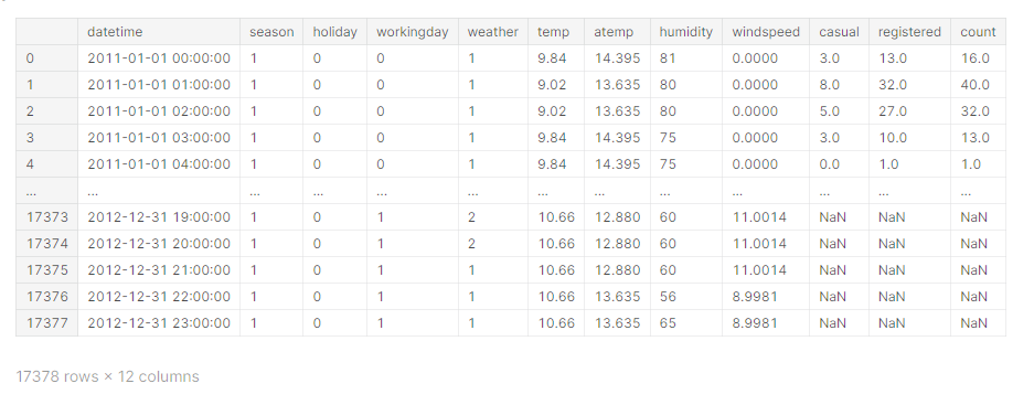
시간 데이터를 쪼개서 피처로 사용
from datetime import datetime

# 날짜 피처 생성
all_data['date'] = all_data['datetime'].apply(lambda x:x.split()[0])
# 연도 피처 생성
all_data['year'] = all_data['datetime'].apply(lambda x:x.split()[0].split("-")[0])
# 월 피처 생성
all_data['month'] = all_data['datetime'].apply(lambda x:x.split()[0].split("-")[1])
# 시 피처 생성
all_data['hour'] = all_data['datetime'].apply(lambda x:x.split()[1].split(":")[0])
# 요일 피처 생성
all_data['weekday'] = all_data['date'].apply(lambda dateString : datetime.strptime(dateString, "%Y-%m-%d").weekday()) # 요일을 정수형으로 생성

# train은 1~19일 test는 20 ~ 말일 이므로 사용할 필요가 없음
또한, 쓸모없는 피처들을 제거한다.
month를 3개씩 묶은 feature = season
windspeed, casual 등등..
drop_features = ['casual', 'registered', 'datetime', 'date', 'windspeed', 'month']
all_data = all_data.drop(drop_features, axis=1)
feature 작업을 완료하였으므로 다시 train, test로 나누어준다.
X_train = all_data[~pd.isnull(all_data['count'])]
X_test = all_data[pd.isnull(all_data['count'])]
# 타켓의 count 제거
X_train = X_train.drop(['count'], axis=1)
X_test = X_test.drop(['count'], axis=1)
y = train['count'] # 타켓값X_train.head()

이 대회는 평가를 RMSLE를 통해 점수를 매기므로 RMSLE를 계산하는 함수를 작성해주었다.
import numpy as np
def rmsle(y_true, y_pred, convertExp=True):
    # 지수변환 (count를 로그변환해서 예측하기 때문에 다시 돌려줘야함)
    if convertExp:
        y_true = np.exp(y_true)
        y_pred = np.exp(y_pred)

    # 로그변환 후 결측값을 0으로 변환
    log_true = np.nan_to_num(np.log(y_true+1))
    log_pred = np.nan_to_num(np.log(y_pred+1))

    # RMSLE 계산
    output = np.sqrt(np.mean((log_true - log_pred)**2)) # RMSLE 공식을 그래서 작성
    return output
Linear Regression 이용
from sklearn.linear_model import LinearRegression

linear_reg_model = LinearRegression()

log_y = np.log(y) # 타겟값 로그변환
linear_reg_model.fit(X_train, log_y) # 모델 훈련
linearreg_preds = linear_reg_model.predict(X_test) # 테스트 데이터로 예측
submission['count'] = np.exp(linearreg_preds) # 지수변환
submission.to_csv('submission.csv', index=False) # 파일로 저장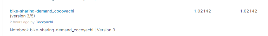
RMSLE는 작을수록 좋은데 1.02142로 매우 좋지 못하게 나왔다.
성능개선을 해보자
릿지(Ridge) 회귀 모델
- 규제(regularization)을 통해 과대적합(overfitting)을 방지를 해주는 모델
from sklearn.linear_model import Ridge
from sklearn.model_selection import GridSearchCV
from sklearn import metrics

ridge_model = Ridge()

# 하이퍼파라미터 값 목록
ridge_params = {'max_iter':[3000], 'alpha':[0.1, 1, 2, 3, 4, 10, 30, 100, 200, 300, 400, 800, 900, 1000]}

# 교차 검증용 평가 함수(RMSLE 점수 계산)
rmsle_scorer = metrics.make_scorer(rmsle, greater_is_better=False)

# 그리드서치(with 릿지) 객체 생성
gridsearch_ridge_model = GridSearchCV(estimator = ridge_model,   # 릿지모델
                                      param_grid = ridge_params, # 값 목록
                                      scoring=rmsle_scorer,      # 평가지표
                                      cv=5)                      # 교차 검증 분할 수


log_y = np.log(y) # 타깃값 로그변환
gridsearch_ridge_model.fit(X_train, log_y) # 훈련 (그리드서치)
GridSearchCV(cv=5, estimator=Ridge(),
param_grid={'alpha': [0.1, 1, 2, 3, 4, 10, 30, 100, 200, 300, 400,
800, 900, 1000],
'max_iter': [3000]},
scoring=make_scorer(rmsle, greater_is_better=False))
print('최적 하이퍼파라미터 : ', gridsearch_ridge_model.best_params_)최적 하이퍼파라미터 : {'alpha': 0.1, 'max_iter': 3000}# 예측
preds = gridsearch_ridge_model.best_estimator_.predict(X_train)
# 평가
print(f"릿지 회귀 RMSLE 값 : {rmsle(log_y, preds, True):.4f}")릿지 회귀 RMSLE 값 : 1.0205
성능개선이 이루어지지 않았다.
라쏘(Lasso) 회귀 모델
from sklearn.linear_model import Lasso

# 모델 생성
lasso_model = Lasso()
# 하이퍼파라미터 값 목록
lasso_alpha = 1/np.array([0.1, 1, 2, 3, 4, 10, 30, 100, 200, 300, 400, 800, 900, 1000])
lasso_params = {'max_iter':[3000], 'alpha':lasso_alpha}

# 그리드서치(with 라쏘) 객체 생성
gridsearch_lasso_model = GridSearchCV(estimator=lasso_model,
                                      param_grid=lasso_params,
                                      scoring=rmsle_scorer,
                                      cv=5)

# 그리드 서치 수행
log_y = np.log(y)
gridsearch_lasso_model.fit(X_train, log_y)

print('최적 하이퍼파라미터 : ', gridsearch_lasso_model.best_params_)
최적 하이퍼파라미터 : {'alpha': 0.00125, 'max_iter': 3000}
# 예측
preds = gridsearch_lasso_model.best_estimator_.predict(X_train)

# 평가
print(f"라쏘 회귀 RMSLE 값 : {rmsle(log_y, preds, True):.4f}")
라쏘 회귀 RMSLE 값 : 1.0205역시 좋지 못한 결과를 보여준다.
RandomForest (랜덤포레스트) 회귀 모델
from sklearn.ensemble import RandomForestRegressor

# 모델 생성
randomforest_model = RandomForestRegressor()
# 그리드서치 객체 생성
rf_params = {'random_state':[42], 'n_estimators':[100, 120, 140]}
gridsearch_random_forest_model = GridSearchCV(estimator=randomforest_model,
                                              param_grid=rf_params,
                                              scoring=rmsle_scorer,
                                              cv=5)

# 그리드서치 수행
log_y = np.log(y)
gridsearch_random_forest_model.fit(X_train, log_y)
print("최적 하이퍼파라미터 : ", gridsearch_random_forest_model.best_params_)
최적 하이퍼파라미터 : {'n_estimators': 140, 'random_state': 42}
# 예측
preds = gridsearch_random_forest_model.best_estimator_.predict(X_train)

# 평가
print(f"랜덤 포레스트 회귀 RMSLE 값 : {rmsle(log_y, preds, True):.4f}")
랜덤 포레스트 회귀 RMSLE 값 : 0.1127훨씬 개선된 모습을 확인할 수 있다.
주의!!
지금은 학습데이터를 통해서 RMSLE에 넣어서 확인해보고 있는데 이는 사실 잘못된 검증 방법이다.
검증데이터는 학습데이터가 아닌 검증데이터를 따로 구성해서 확인하는 것이 원칙이다.
import seaborn as sns
import matplotlib.pyplot as plt

randomforest_preds = gridsearch_random_forest_model.best_estimator_.predict(X_test)

figure, axes = plt.subplots(ncols=2)
figure.set_size_inches(10, 4)

sns.histplot(y, bins=50, ax=axes[0])
axes[0].set_title('Train Data Distribution')
sns.histplot(np.exp(randomforest_preds), bins=50, ax=axes[1])
axes[1].set_title('Predicted Test Data Distribution')
두 그래프가 비슷하게 분포되어있음을 확인
submission['count'] = np.exp(randomforest_preds) # 지수변환
submission.to_csv('submission.csv', index=False)
그 결과는
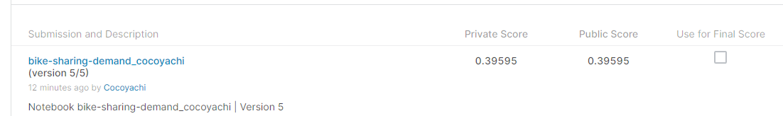

7년 전 대회라 대쉬보드에 제출은 할 수 없지만 대략 195등 정도의 높은 점수를 받을 수 있다.
728x90
반응형
'프로젝트 > Bike Sharing Demand' 카테고리의 다른 글
| [Kaggle]Bike Sharing Demand 데이터 살펴보기(그래프그리기) (0) | 2022.07.17 |
|---|